
Notice
Recent Posts
Recent Comments
Link
| 일 | 월 | 화 | 수 | 목 | 금 | 토 |
|---|---|---|---|---|---|---|
| 1 | 2 | 3 | 4 | |||
| 5 | 6 | 7 | 8 | 9 | 10 | 11 |
| 12 | 13 | 14 | 15 | 16 | 17 | 18 |
| 19 | 20 | 21 | 22 | 23 | 24 | 25 |
| 26 | 27 | 28 | 29 | 30 | 31 |
Tags
- 데이터사이언스
- OpenCV
- gray level resolution
- 이미지향상
- 고차원데이터
- 이미지처리
- 데이터분석
- OMSA
- 이미지콘볼루션
- Data Analysis
- high-dimensional data analysis
- 이미지분석
- datascience
- 이미지대비
- data science
- high dimensional data analysis
- bitdepth
- 고차원데이터분석
- 함수형데이터분석
- 미국온라인석사
- 이미지변환
- 모델링
- 빅데이터
- big data
- functional data analysis
- simulation
- 시뮬레이션
- 스플라인
- 이미지프로세싱
- 이미지스트레칭
Archives
- Today
- Total
곤약노트
이미지 변환 (Image Transformation) ①임계값 처리 (Thresholding)로 흑백 이미지 만들기 본문
Data Science/High-Dimensional Data Analytics
이미지 변환 (Image Transformation) ①임계값 처리 (Thresholding)로 흑백 이미지 만들기
곤약처럼 부드럽게, 쫀쫀하게 2025. 6. 26. 09:00디지털 이미지 처리의 가장 기본적인 변환 방법 중 하나는 바로 임계값 처리(Thresholding)입니다. 이 방법은 회색조(grayscale) 이미지를 흑백(black & white) 이미지로 바꿔주는 간단하면서도 매우 유용한 기법입니다.
회색조(grayscale) ▶ Thresholing ▶ 흑백(black & white)
Thresholding이란?
임계값 처리란, 픽셀의 밝기 값이 어떤 기준 값(임계값 p)보다 크면 흰색(1)으로, 작거나 같으면 검은색(0)으로 이진화(Binarization) 시키는 방식입니다.
$$ g(x, y) = T(f(x, y)) = \begin{cases} 1 & \text{if } f(x, y) > p \\ 0 & \text{if } f(x, y) \leq p \end{cases} $$
- f(x,y): 원본 이미지에서 (x, y) 위치의 픽셀 밝기
- g(x,y): 변환된 출력 이미지
- p: 기준이 되는 임계값 (threshold)
- 수식에 따라 f(x,y)가 p보다 크면 흰색(1), 아니면 검정색(0)
import cv2
import matplotlib.pyplot as plt

# 1. 이미지 불러오기 (흑백 모드)
image = cv2.imread('watermelon.jpg', cv2.IMREAD_GRAYSCALE)

# 2. 임계값 처리 (Thresholding)
threshold_value = 127
_, binary_image = cv2.threshold(image, threshold_value, 255, cv2.THRESH_BINARY)

# 3. 이미지 및 히스토그램 시각화
plt.figure(figsize=(12, 5))

# 그레이스케일 이미지
plt.subplot(1, 3, 1)
plt.imshow(gray, cmap='gray')
plt.title('Grayscale Image')
plt.axis('off')

# 임계값 처리 이미지
plt.subplot(1, 3, 2)
plt.title(f"Thresholded (p = {threshold_value})")
plt.imshow(binary_image, cmap='gray')
plt.axis('off')

# 히스토그램
plt.subplot(1, 3, 3)
plt.hist(binary_image.ravel(), bins=256, range=[0, 256])
plt.title('Histogram')
plt.xlabel('Pixel Intensity (0~255)')
plt.ylabel('Frequency')

plt.tight_layout()
plt.show()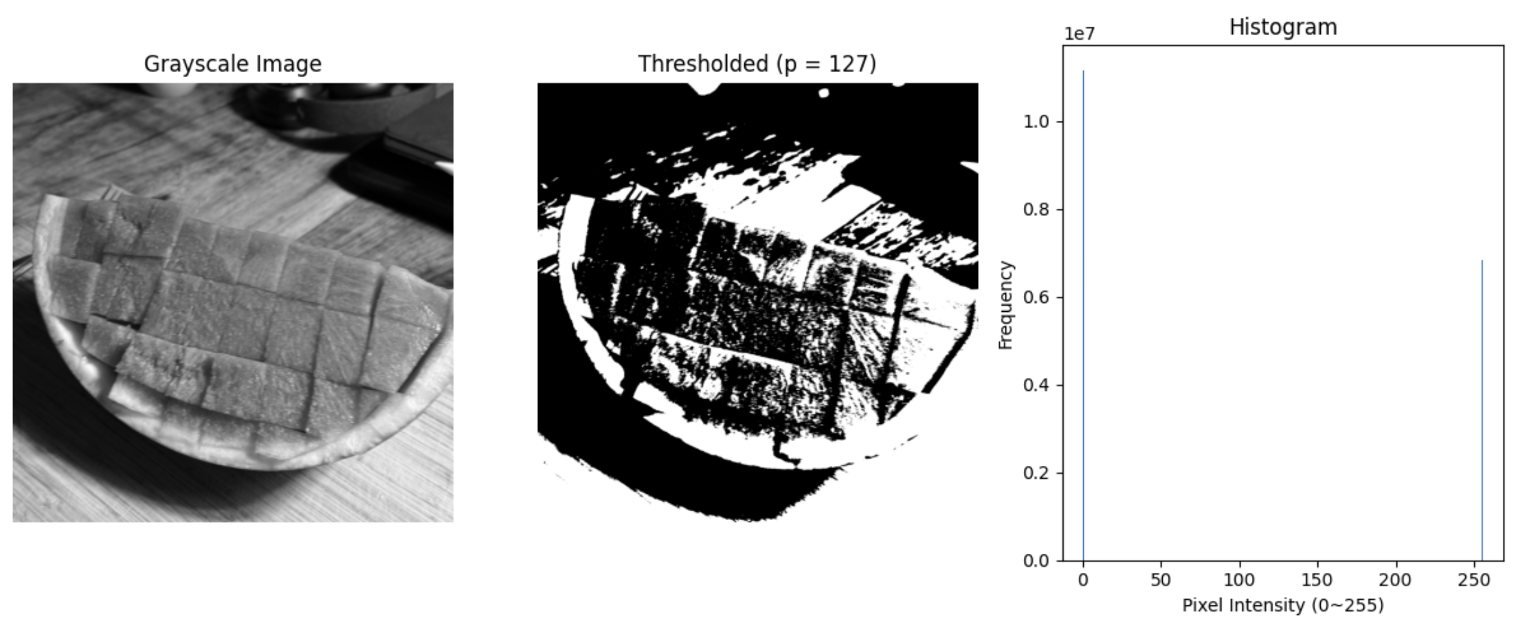

'Data Science > High-Dimensional Data Analytics' 카테고리의 다른 글
'Data Science/High-Dimensional Data Analytics' Related Articles
more


